We can help understand data by building mathematical models, this is key to machine learning.
One of such models is linear regression, in which we fit a line to (x,y) data.
Linear regression fits a straight line through your data. The line has a slope and an intercept, and the model learns both by looking at the error it makes on every point.
It is the first model you should fit. If the relationship in your data is not a straight line, you will see it immediately in the plot.
There are many modules for Machine Learning in Python, but scikit-learn is a popular one.
Linear Regression
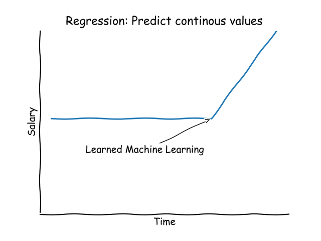
You may want to predict continous values. That is a regression problem. Linear Regression is one of the methods to solve that.
All kinds of values are continous: temperature, salary, numbers and many more. Regression is not always linear, as shown in the image below:
But there are many data points on which linear regression can be applied. Like tay fare, where hours driven is directly correlated with the price to pay.
Modules
Install the required modules;
sudo pip install matplotlib
sudo pip install scikit-learn
sudo pip install scipy
linear regression example
Then we start with a basic plot:
import matplotlib
matplotlib.use('qt5agg')

import matplotlib.pyplot as plt
import numpy as np

randomNumberGenerator = np.random.RandomState(1000)
x = 4 * randomNumberGenerator.rand(100)
y = 4 * x - 1 + randomNumberGenerator.randn(100)
plt.scatter(x, y);
plt.show()
This will create a bunch of random data, which follows a linear path.
In a real life situation, you would use real world data instead of random numbers
We then use the model linear regression from the scikit-learn module.
model = LinearRegression(fit_intercept=True)
model.fit(x[:, np.newaxis], y)
then we define the linear space and predict the y values using the model.
xfit = np.linspace(0, 5, 50)
yfit = model.predict(xfit[:, np.newaxis])
finally we plot the data, summarizing with this code:# pythonprogramminglanguage.com
from sklearn.linear_model import LinearRegression
import matplotlib
matplotlib.use('qt5agg')
import matplotlib.pyplot as plt
import numpy as np
# Create random data
randomNumberGenerator = np.random.RandomState(1000)
x = 4 * randomNumberGenerator.rand(100)
y = 4 * x - 1 + randomNumberGenerator.randn(100)
# Create model
model = LinearRegression(fit_intercept=True)
model.fit(x[:, np.newaxis], y)
xfit = np.linspace(0, 5, 50)
yfit = model.predict(xfit[:, np.newaxis])
# plot
plt.scatter(x, y)
plt.plot(xfit, yfit);
plt.show()
Then we find the fitting line.
The steps
from sklearn.linear_model import LinearRegressionmodel = LinearRegression()model.fit(X, y)where X is two dimensional, one row per sample and one column per feature.model.coef_holds the slope of each feature,model.intercept_the intercept.model.predict([[x]])gives you the prediction.model.score(X, y)gives you R squared, from 0 to 1.
With one feature the formula is just y = slope * x + intercept, and
those two numbers are exactly what least squares gives you.
Check the plot first. If the points curve, a straight line is the wrong model and you want polynomial features or a different algorithm. If R squared is high on the training data and low on the test data, the model is overfitting.
If you want to try this yourself, the exercises on PyChallenge turn the same idea into a few short problems with instant feedback.